深度学习
深度学习应用领域
- 图像识别:IMAGENET
- 机器翻译:Google神经机器翻译系统
- 玩游戏: DeepMind团队开发的自我学习玩游戏的系统
- 语音识别
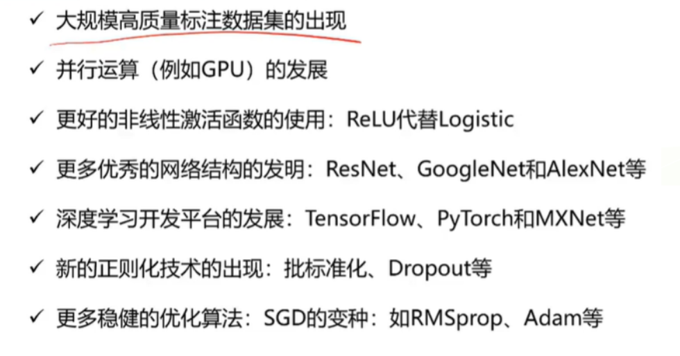
深度学习发展原因
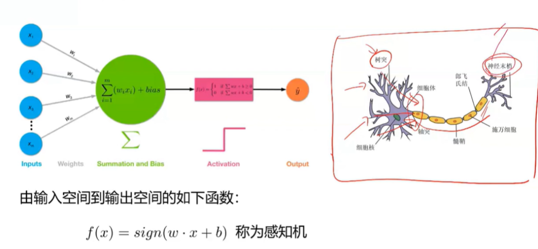
神经元与感知机
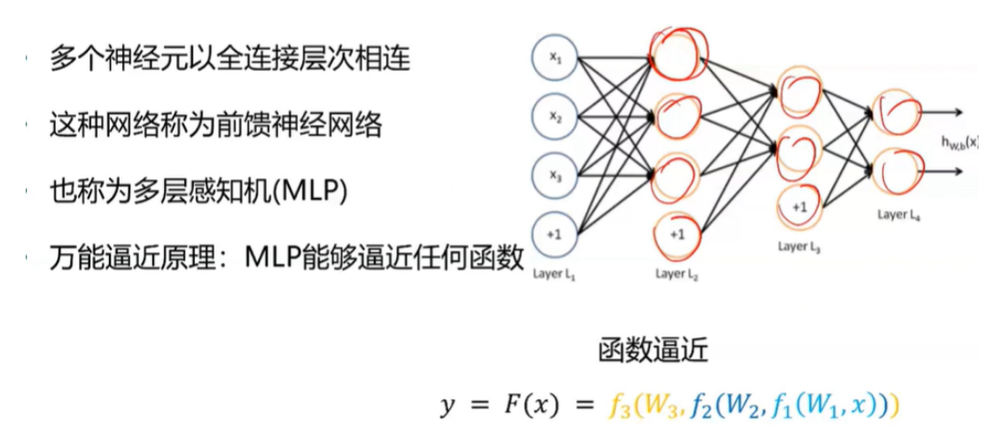
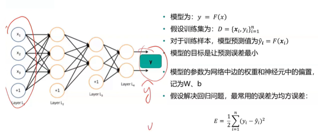
多层感知机(MLP)
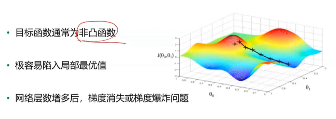
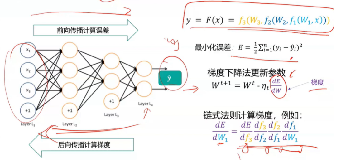
后向传播BP
机器学习 vs 深度学习
- 机器学习需要人工选取特征;深度学习会自动学习有用的特征
- 可以将深度学习视为非线性函数逼近器:深度学习通过一种深层网络结构,实现复杂函数逼近。
- 万能逼近原理:当隐层节点数目足够多时,具有一个隐层的神经网络,可以以任意精度逼近任意具有有限间断点的函数。
- 网络层数越多,需要的隐含节点数目指数减小。
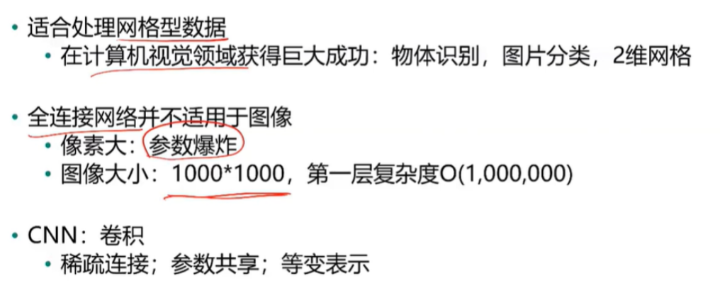
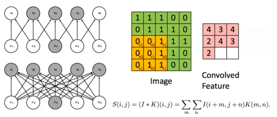
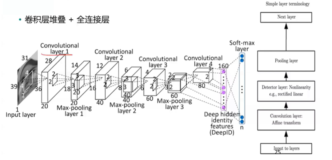
CNN卷积神经网络
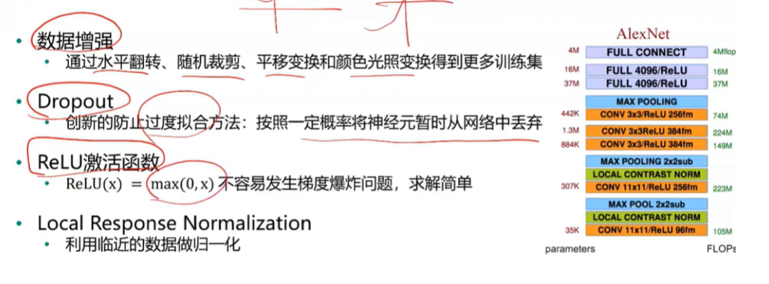
AlexNet
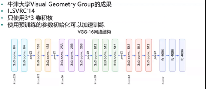
VGG
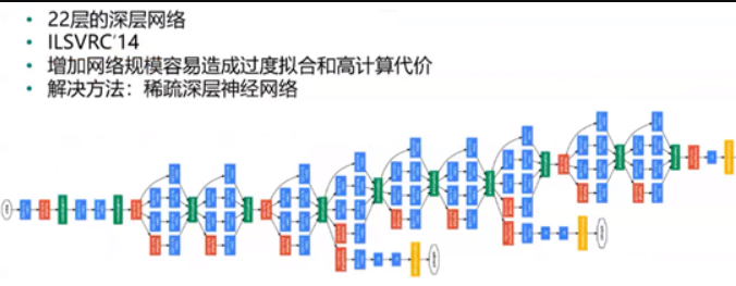
GoogleNet
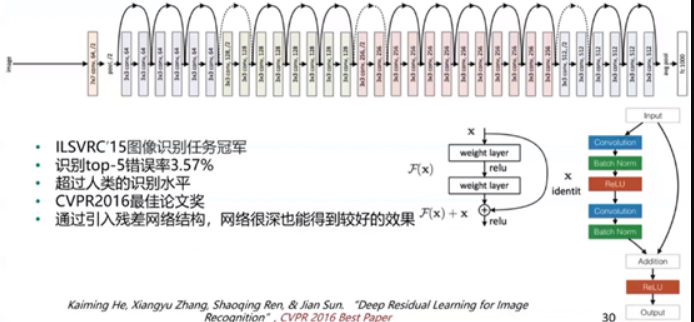
ResNet
RNN 和 GAN
- RNN 适合处理训练型数据:自然语言处理等领域
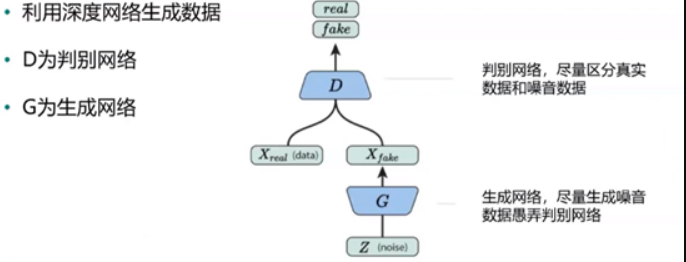
- GAN
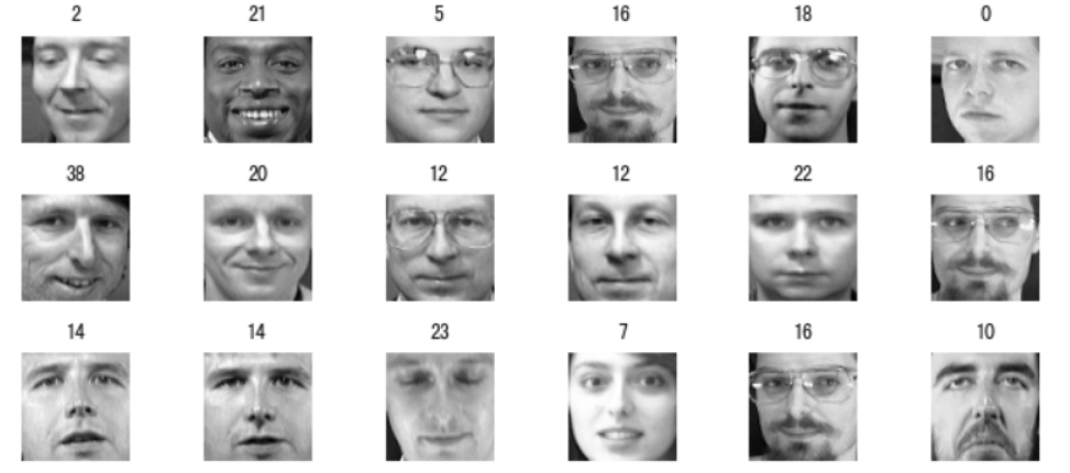
基于卷积神经网络的人脸识别
#使用sklearn的datasets模块在线获取Olivetti Faces数据集。
from sklearn.datasets import fetch_olivetti_faces
faces = fetch_olivetti_faces()
#打印
faces

#数据结构与类型
print("The shape of data:",faces.data.shape, "The data type of data:",type(faces.data))
print("The shape of images:",faces.images.shape, "The data type of images:",type(faces.images))
print("The shape of target:",faces.target.shape, "The data type of target:",type(faces.target))

#使用matshow输出部分人脸图片
import numpy as np
rndperm = np.random.permutation(len(faces.images)) #将数据的索引随机打乱
import matplotlib.pyplot as plt
%matplotlib inline
plt.gray()
fig = plt.figure(figsize=(9,4) )
for i in range(0,18):
    ax = fig.add_subplot(3,6,i+1 )
    plt.title(str(faces.target[rndperm[i]])) #类标
    ax.matshow(faces.images[rndperm[i],:]) #图片内容
    plt.box(False) #去掉边框
    plt.axis("off")#不显示坐标轴
plt.tight_layout()
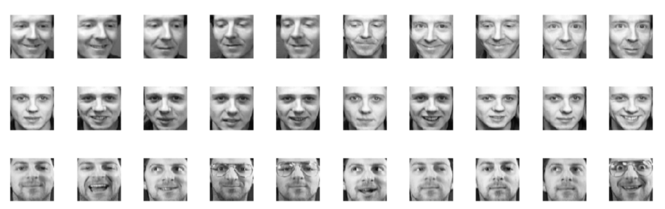
#查看同一个人的不同人脸特点
labels = [2,11,6] #选取三个人
%matplotlib inline
plt.gray()
fig = plt.figure(figsize=(12,4) )
for i in range(0,3):
    faces_labeli = faces.images[faces.target == labels[i]]
    for j in range(0,10):
        ax = fig.add_subplot(3,10,10*i + j+1 )
        ax.matshow(faces_labeli[j])
        plt.box(False) #去掉边框
        plt.axis("off")#不显示坐标轴
plt.tight_layout()
#将数据集划分为训练集和测试集两部分,注意要按照图像标签进行分层采样
# 定义特征和标签
X,y = faces.images,faces.target
# 以5:5比例随机地划分训练集和测试集
from sklearn.model_selection import train_test_split
train_x, test_x, train_y, test_y = train_test_split(X, y, test_size=0.5,stratify = y,random_state=0)
# 记录测试集中出现的类别,后期模型评价画混淆矩阵时需要
#index = set(test_y)

# 转换数据维度,模型训练时要用
train_x = train_x.reshape(train_x.shape[0], 64, 64, 1)
test_x = test_x.reshape(test_x.shape[0], 64, 64, 1)
#从keras的相应模块引入需要的对象。
import warnings
warnings.filterwarnings('ignore') #该行代码的作用是隐藏警告信息
import tensorflow as tf
import tensorflow.keras.layers as layers
import tensorflow.keras.backend as K
K.clear_session()
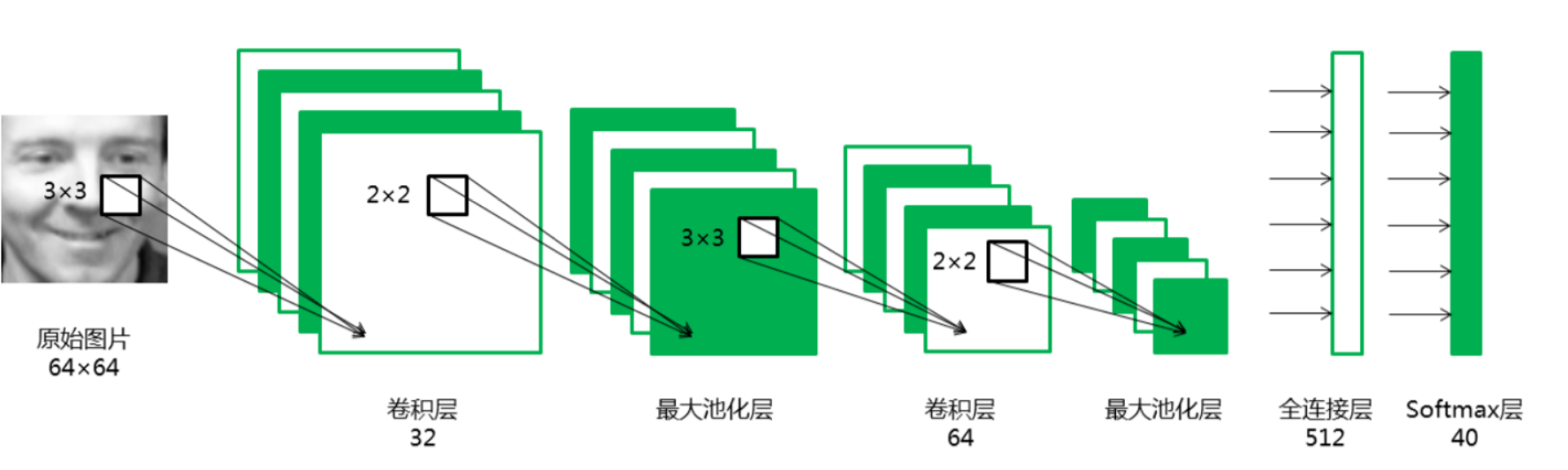
#逐层搭建卷积神经网络模型。此处使用了函数式api
inputs = layers.Input(shape=(64,64,1), name='inputs')
conv1 = layers.Conv2D(32,3,3,padding="same",activation="relu",name="conv1")(inputs) #卷积层32
maxpool1 = layers.MaxPool2D(pool_size=(2,2),name="maxpool1")(conv1) #池化层1
conv2 = layers.Conv2D(64,3,3,padding="same",activation="relu",name="conv2")(maxpool1) #卷积层64
maxpool2 = layers.MaxPool2D(pool_size=(2,2),name="maxpool2")(conv2) #池化层2
flatten1 = layers.Flatten(name="flatten1")(maxpool2) #拉成一维
dense1 = layers.Dense(512,activation="tanh",name="dense1")(flatten1)
dense2 = layers.Dense(40,activation="softmax",name="dense2")(dense1) #40个分类
model = tf.keras.Model(inputs,dense2)
#网络结构打印。
model.summary()
#模型编译,指定误差函数、优化方法和评价指标。使用训练集进行模型训练。
model.compile(loss='sparse_categorical_crossentropy', optimizer="Adam", metrics=['accuracy'])
model.fit(train_x,train_y, batch_size=20, epochs=30, validation_data=(test_x,test_y),verbose=2)
#评价
score = model.evaluate(test_x, test_y)
print('Test loss:', score[0])
print('Test accuracy:', score[1])
#数据增强——ImageDataGenerator
from tensorflow.keras.preprocessing.image import ImageDataGenerator
# 定义随机变换的类别及程度
datagen = ImageDataGenerator(
rotation_range=0, # 图像随机转动的角度
width_shift_range=0.01, # 图像水平偏移的幅度
height_shift_range=0.01, # 图像竖直偏移的幅度
shear_range=0.01, # 逆时针方向的剪切变换角度
zoom_range=0.01, # 随机缩放的幅度
horizontal_flip=True,
fill_mode='nearest')
#使用增强后的数据进行模型训练与评价
inputs = layers.Input(shape=(64,64,1), name='inputs')
conv1 = layers.Conv2D(32,3,3,padding="same",activation="relu",name="conv1")(inputs)
maxpool1 = layers.MaxPool2D(pool_size=(2,2),name="maxpool1")(conv1)
conv2 = layers.Conv2D(64,3,3,padding="same",activation="relu",name="conv2")(maxpool1)
maxpool2 = layers.MaxPool2D(pool_size=(2,2),name="maxpool2")(conv2)
flatten1 = layers.Flatten(name="flatten1")(maxpool2)
dense1 = layers.Dense(512,activation="tanh",name="dense1")(flatten1)
dense2 = layers.Dense(40,activation="softmax",name="dense2")(dense1)
model2 = tf.keras.Model(inputs,dense2)
model2.compile(loss='sparse_categorical_crossentropy', optimizer="Adam", metrics=['accuracy'])
# 训练模型
model2.fit_generator(datagen.flow(train_x, train_y, batch_size=200),epochs=30,steps_per_epoch=16, verbose = 2,validation_data=(test_x,test_y))
# 模型评价
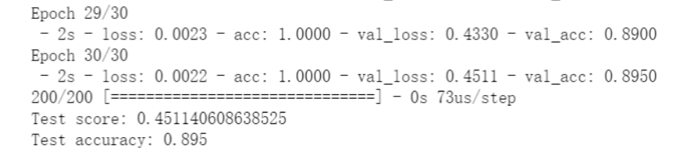
score = model2.evaluate(test_x, test_y)
print('Test score:', score[0])
print('Test accuracy:', score[1])