翻译自《Demo Week: Time Series Machine Learning with timetk》
原文链接:www.business-science.io/code-tools/2017/10/24/demo_week_timetk.html
时间序列分析工具箱——timetk

timetk 的主要用途
三个主要用途:
- 时间序列机器学习:使用回归算法进行预测;
- 构造时间序列索引:基于时间模式提取、探索和扩展时间序列索引;
- 转换不同类型的时间序列数据(例如
tbl、xts、zoo、ts之间):轻松实现不同类型的时间序列数据之间的相互转换。
我们今天将讨论时间序列机器学习和数据类型转换。第二个议题(提取和构造未来时间序列)将在时间序列机器学习中涉及,因为这对预测准确性非常关键。
加载包
需要加在两个包:
tidyquant:用于获取数据并在后台加载 tidyversetimetk:R 中用于处理时间序列的工具包
如果还没有安装过,请用下面的命令安装:
# Install packages
install.packages("timetk")
install.packages("tidyquant")
加载包。
# Load libraries
library(timetk)     # Toolkit for working with time series in R
library(tidyquant)  # Loads tidyverse, financial pkgs, used to get data
数据
我们将使用 tidyquant 中的 tq_get() 函数从 FRED 获取数据——啤酒、葡萄酒和蒸馏酒销售数据。
# Beer, Wine, Distilled Alcoholic Beverages, in Millions USD
beer_sales_tbl <- tq_get(
    "S4248SM144NCEN",
    get = "economic.data",
    from = "2010-01-01",
    to = "2016-12-31")

beer_sales_tbl
## # A tibble: 84 x 2
##          date price
##        <date> <int>
##  1 2010-01-01  6558
##  2 2010-02-01  7481
##  3 2010-03-01  9475
##  4 2010-04-01  9424
##  5 2010-05-01  9351
##  6 2010-06-01 10552
##  7 2010-07-01  9077
##  8 2010-08-01  9273
##  9 2010-09-01  9420
## 10 2010-10-01  9413
## # ... with 74 more rows
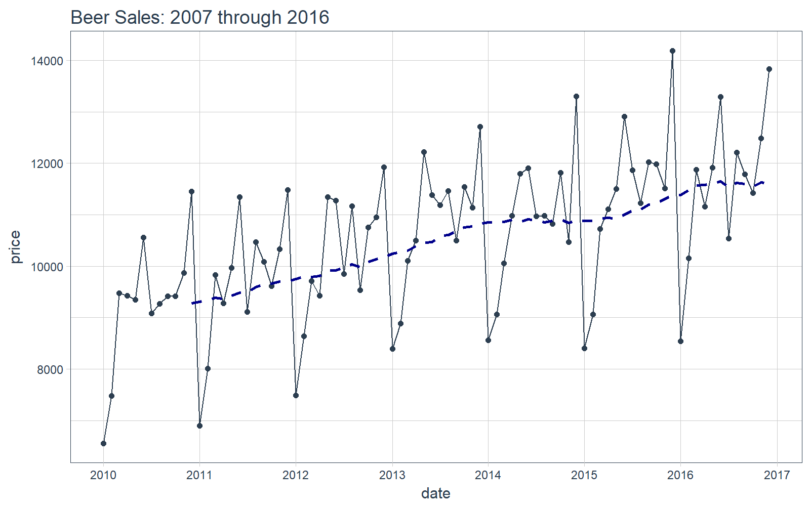
可视化数据是一个好东西,这有助于帮助我们了解正在使用的是什么数据。可视化对于时间序列分析和预测尤为重要。我们将使用 tidyquant 画图工具:主要是用 geom_ma(ma_fun = SMA,n = 12) 来添加一个周期为 12 的简单移动平均线来了解趋势。我们还可以看到似乎同时存在着趋势性(移动平均线以近似线性的模式增长)和季节性(波峰和波谷倾向于在特定月份发生)。
# Plot Beer Sales
beer_sales_tbl %>%
    ggplot(aes(date, price)) +
    geom_line(col = palette_light()[1]) +
    geom_point(col = palette_light()[1]) +
    geom_ma(ma_fun = SMA, n = 12, size = 1) +
    theme_tq() +
    scale_x_date(date_breaks = "1 year", date_labels = "%Y") +
    labs(title = "Beer Sales: 2007 through 2016")
现在你对我们要分析的时间序列有了直观的感受,那么让我们继续!
timetk 教程:
教程分为两部分。首先,我们将遵循时间序列机器学习的工作流程。其次,我们将介绍数据转换工具。
PART 1:时间序列机器学习
时间序列机器学习是预测时间序列数据的一种很好的方法,但在我们开始之前,这里有几个注意点:
- 关键洞察力:将时间序列签名(时间戳信息按列扩展到特征集)用于执行机器学习。
- 目标:我们将使用时间序列签名预测未来 12 个月的时间序列数据。
我们将遵循可用于执行时间序列机器学习的工作流程。你将看到几个 timetk 函数如何帮助完成此过程。我们将使用简单的 lm() 线性回归进行机器学习,你将看到使用时间序列签名会使机器学习更强大和准确。此外,你还应该考虑使用其他更强大的机器学习算法,例如 xgboost、glmnet(LASSO)等。
STEP 0:回顾数据
看看我们的起点,先打印出 beer_sales_tbl。
# Starting point
beer_sales_tbl
## # A tibble: 84 x 2
##          date price
##        <date> <int>
##  1 2010-01-01  6558
##  2 2010-02-01  7481
##  3 2010-03-01  9475
##  4 2010-04-01  9424
##  5 2010-05-01  9351
##  6 2010-06-01 10552
##  7 2010-07-01  9077
##  8 2010-08-01  9273
##  9 2010-09-01  9420
## 10 2010-10-01  9413
## # ... with 74 more rows
我们可以使用 tk_index() 来提取索引;使用 tk_get_timeseries_summary() 来检索索引的摘要信息,进而快速了解时间序列。我们使用 glimpse() 输出一个更漂亮的格式。
beer_sales_tbl %>%
    tk_index() %>%
    tk_get_timeseries_summary() %>%
    glimpse()
## Observations: 1
## Variables: 12
## $ n.obs        <int> 84
## $ start        <date> 2010-01-01
## $ end          <date> 2016-12-01
## $ units        <chr> "days"
## $ scale        <chr> "month"
## $ tzone        <chr> "UTC"
## $ diff.minimum <dbl> 2419200
## $ diff.q1      <dbl> 2592000
## $ diff.median  <dbl> 2678400
## $ diff.mean    <dbl> 2629475
## $ diff.q3      <dbl> 2678400
## $ diff.maximum <dbl> 2678400
你可以看到一些重要的特征,例如起始、结束、单位等等。还有时间差的分位数(相邻两个观察之间差距的秒数),这对评估规律性的程度很有用。由于时间尺度是月度的,因此每个月之间差距的秒数并不规则。
STEP 1:扩充时间序列签名
tk_augment_timeseries_signature() 函数将时间戳信息逐列扩展到机器学习特征集中,并将时间序列信息列添加到初始数据表。
# Augment (adds data frame columns)
beer_sales_tbl_aug <- beer_sales_tbl %>%
    tk_augment_timeseries_signature()

beer_sales_tbl_aug
## # A tibble: 84 x 30
##          date price  index.num    diff  year year.iso  half quarter
##        <date> <int>      <int>   <int> <int>    <int> <int>   <int>
##  1 2010-01-01  6558 1262304000      NA  2010     2009     1       1
##  2 2010-02-01  7481 1264982400 2678400  2010     2010     1       1
##  3 2010-03-01  9475 1267401600 2419200  2010     2010     1       1
##  4 2010-04-01  9424 1270080000 2678400  2010     2010     1       2
##  5 2010-05-01  9351 1272672000 2592000  2010     2010     1       2
##  6 2010-06-01 10552 1275350400 2678400  2010     2010     1       2
##  7 2010-07-01  9077 1277942400 2592000  2010     2010     2       3
##  8 2010-08-01  9273 1280620800 2678400  2010     2010     2       3
##  9 2010-09-01  9420 1283299200 2678400  2010     2010     2       3
## 10 2010-10-01  9413 1285891200 2592000  2010     2010     2       4
## # ... with 74 more rows, and 22 more variables: month <int>,
## #   month.xts <int>, month.lbl <ord>, day <int>, hour <int>,
## #   minute <int>, second <int>, hour12 <int>, am.pm <int>,
## #   wday <int>, wday.xts <int>, wday.lbl <ord>, mday <int>,
## #   qday <int>, yday <int>, mweek <int>, week <int>, week.iso <int>,
## #   week2 <int>, week3 <int>, week4 <int>, mday7 <int>
STEP 2:模型
任何回归模型都可以应用于数据,我们在这里使用 lm()。 请注意,我们删除了 date 和 diff 列。大多数算法无法使用日期数据,而 diff 列对机器学习没有什么用处(它对于查找数据中的时间间隔更有用)。
# linear regression model used, but can use any model
fit_lm <- lm(
    price ~ .,
    data = select(
        beer_sales_tbl_aug,
        -c(date, diff)))

summary(fit_lm)
##
## Call:
## lm(formula = price ~ ., data = select(beer_sales_tbl_aug, -c(date,
##     diff)))
##
## Residuals:
##    Min     1Q Median     3Q    Max
## -447.3 -145.4  -18.2  169.8  421.4
##
## Coefficients: (16 not defined because of singularities)
##                Estimate Std. Error t value Pr(>|t|)
## (Intercept)   3.660e+08  1.245e+08   2.940 0.004738 **
## index.num     5.900e-03  2.003e-03   2.946 0.004661 **
## year         -1.974e+05  6.221e+04  -3.173 0.002434 **
## year.iso      1.159e+04  6.546e+03   1.770 0.082006 .
## half         -2.132e+03  6.107e+02  -3.491 0.000935 ***
## quarter      -1.239e+04  2.190e+04  -0.566 0.573919
## month        -3.910e+03  7.355e+03  -0.532 0.597058
## month.xts            NA         NA      NA       NA
## month.lbl.L          NA         NA      NA       NA
## month.lbl.Q  -1.643e+03  2.069e+02  -7.942 8.59e-11 ***
## month.lbl.C   8.368e+02  5.139e+02   1.628 0.108949
## month.lbl^4   6.452e+02  1.344e+02   4.801 1.18e-05 ***
## month.lbl^5   7.563e+02  4.241e+02   1.783 0.079852 .
## month.lbl^6   3.206e+02  1.609e+02   1.992 0.051135 .
## month.lbl^7  -3.537e+02  1.867e+02  -1.894 0.063263 .
## month.lbl^8   3.687e+02  3.217e+02   1.146 0.256510
## month.lbl^9          NA         NA      NA       NA
## month.lbl^10  6.339e+02  2.240e+02   2.830 0.006414 **
## month.lbl^11         NA         NA      NA       NA
## day                  NA         NA      NA       NA
## hour                 NA         NA      NA       NA
## minute               NA         NA      NA       NA
## second               NA         NA      NA       NA
## hour12               NA         NA      NA       NA
## am.pm                NA         NA      NA       NA
## wday         -8.264e+01  1.898e+01  -4.353 5.63e-05 ***
## wday.xts             NA         NA      NA       NA
## wday.lbl.L           NA         NA      NA       NA
## wday.lbl.Q   -7.109e+02  1.093e+02  -6.503 2.13e-08 ***
## wday.lbl.C    2.355e+02  1.336e+02   1.763 0.083273 .
## wday.lbl^4    8.033e+01  1.133e+02   0.709 0.481281
## wday.lbl^5    6.480e+01  8.029e+01   0.807 0.422951
## wday.lbl^6    2.276e+01  8.200e+01   0.278 0.782319
## mday                 NA         NA      NA       NA
## qday         -1.362e+02  2.418e+02  -0.563 0.575326
## yday         -2.356e+02  1.416e+02  -1.664 0.101627
## mweek        -1.670e+02  1.477e+02  -1.131 0.262923
## week         -1.764e+02  1.890e+02  -0.933 0.354618
## week.iso      2.315e+02  1.256e+02   1.842 0.070613 .
## week2        -1.235e+02  1.547e+02  -0.798 0.428283
## week3                NA         NA      NA       NA
## week4                NA         NA      NA       NA
## mday7                NA         NA      NA       NA
## ---
## Signif. codes:  0 '***' 0.001 '**' 0.01 '*' 0.05 '.' 0.1 ' ' 1
##
## Residual standard error: 260.4 on 57 degrees of freedom
## Multiple R-squared:  0.9798,	Adjusted R-squared:  0.9706
## F-statistic: 106.4 on 26 and 57 DF,  p-value: < 2.2e-16
STEP 3:构建未来(新)数据
使用 tk_index() 来扩展索引。
# Retrieves the timestamp information
beer_sales_idx <- beer_sales_tbl %>%
    tk_index()

tail(beer_sales_idx)
## [1] "2016-07-01" "2016-08-01" "2016-09-01" "2016-10-01" "2016-11-01"
## [6] "2016-12-01"
通过 tk_make_future_timeseries 函数从现有索引构造未来索引。函数会在内部检查索引的周期性,并返回正确的序列。我们在 whole vignette on how to make future time series 介绍了该主题更详尽的内容。
# Make future index
future_idx <- beer_sales_idx %>%
    tk_make_future_timeseries(
        n_future = 12)

future_idx
##  [1] "2017-01-01" "2017-02-01" "2017-03-01" "2017-04-01" "2017-05-01"
##  [6] "2017-06-01" "2017-07-01" "2017-08-01" "2017-09-01" "2017-10-01"
## [11] "2017-11-01" "2017-12-01"
用 tk_get_timeseries_signature() 将未来索引转换成时间序列签名数据框。
new_data_tbl <- future_idx %>%
    tk_get_timeseries_signature()

new_data_tbl
## # A tibble: 12 x 29
##         index  index.num    diff  year year.iso  half quarter month
##        <date>      <int>   <int> <int>    <int> <int>   <int> <int>
##  1 2017-01-01 1483228800      NA  2017     2016     1       1     1
##  2 2017-02-01 1485907200 2678400  2017     2017     1       1     2
##  3 2017-03-01 1488326400 2419200  2017     2017     1       1     3
##  4 2017-04-01 1491004800 2678400  2017     2017     1       2     4
##  5 2017-05-01 1493596800 2592000  2017     2017     1       2     5
##  6 2017-06-01 1496275200 2678400  2017     2017     1       2     6
##  7 2017-07-01 1498867200 2592000  2017     2017     2       3     7
##  8 2017-08-01 1501545600 2678400  2017     2017     2       3     8
##  9 2017-09-01 1504224000 2678400  2017     2017     2       3     9
## 10 2017-10-01 1506816000 2592000  2017     2017     2       4    10
## 11 2017-11-01 1509494400 2678400  2017     2017     2       4    11
## 12 2017-12-01 1512086400 2592000  2017     2017     2       4    12
## # ... with 21 more variables: month.xts <int>, month.lbl <ord>,
## #   day <int>, hour <int>, minute <int>, second <int>, hour12 <int>,
## #   am.pm <int>, wday <int>, wday.xts <int>, wday.lbl <ord>,
## #   mday <int>, qday <int>, yday <int>, mweek <int>, week <int>,
## #   week.iso <int>, week2 <int>, week3 <int>, week4 <int>,
## #   mday7 <int>
STEP 4:预测新数据
将 predict() 应用于回归模型。注意,和之前使用 lm() 函数时一样,去掉 index 和 diff 列。
# Make predictions
pred <- predict(
    fit_lm,
    newdata = select(
        new_data_tbl, -c(index, diff)))

predictions_tbl <- tibble(
    date  = future_idx,
    value = pred)

predictions_tbl
## # A tibble: 12 x 2
##          date     value
##        <date>     <dbl>
##  1 2017-01-01  9509.122
##  2 2017-02-01 10909.189
##  3 2017-03-01 12281.835
##  4 2017-04-01 11378.678
##  5 2017-05-01 13080.710
##  6 2017-06-01 13583.471
##  7 2017-07-01 11529.085
##  8 2017-08-01 12984.939
##  9 2017-09-01 11859.998
## 10 2017-10-01 12331.419
## 11 2017-11-01 13047.033
## 12 2017-12-01 13940.003
STEP 5:比较实际值与预测值
我们可以使用 tq_get() 来检索实际数据。注意,我们没有用于比较的完整数据,但我们至少可以比较前几个月的实际值。
actuals_tbl <- tq_get(
    "S4248SM144NCEN",
    get = "economic.data",
    from = "2017-01-01",
    to = "2017-12-31")
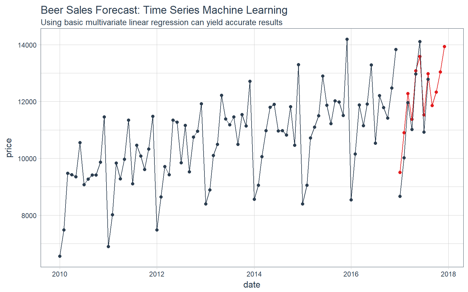
可视化我们的预测。
# Plot Beer Sales Forecast
beer_sales_tbl %>%
    ggplot(aes(x = date, y = price)) +
    # Training data
    geom_line(color = palette_light()[[1]]) +
    geom_point(color = palette_light()[[1]]) +
    # Predictions
    geom_line(
        aes(y = value),
        color = palette_light()[[2]],
        data = predictions_tbl) +
    geom_point(
        aes(y = value),
        color = palette_light()[[2]],
        data = predictions_tbl) +
    # Actuals
    geom_line(
        color = palette_light()[[1]],
        data = actuals_tbl) +
    geom_point(
        color = palette_light()[[1]],
        data = actuals_tbl) +
    # Aesthetics
    theme_tq() +
    labs(
        title = "Beer Sales Forecast: Time Series Machine Learning",
        subtitle = "Using basic multivariate linear regression can yield accurate results")
我们可以检查测试集上的错误(实际值 vs 预测值)。
# Investigate test error
error_tbl <- left_join(
    actuals_tbl, predictions_tbl) %>%
    rename(
        actual = price, pred = value) %>%
    mutate(
        error     = actual - pred,
        error_pct = error / actual)

error_tbl
## # A tibble: 8 x 5
##         date actual      pred     error    error_pct
##       <date>  <int>     <dbl>     <dbl>        <dbl>
## 1 2017-01-01   8664  9509.122 -845.1223 -0.097544127
## 2 2017-02-01  10017 10909.189 -892.1891 -0.089067495
## 3 2017-03-01  11960 12281.835 -321.8352 -0.026909301
## 4 2017-04-01  11019 11378.678 -359.6777 -0.032641592
## 5 2017-05-01  12971 13080.710 -109.7099 -0.008458092
## 6 2017-06-01  14113 13583.471  529.5292  0.037520667
## 7 2017-07-01  10928 11529.085 -601.0854 -0.055004156
## 8 2017-08-01  12788 12984.939 -196.9386 -0.015400265
接着,我们可以做一些误差度量。预测值和实际值的 MAPE(平均绝对百分误差)接近 4.5%,对于简单的多元线性回归模型来说是相当好的结果。更复杂的算法可以产生更精确的结果。
# Calculating test error metrics
test_residuals <- error_tbl$error
test_error_pct <- error_tbl$error_pct * 100 # Percentage error

me   <- mean(test_residuals, na.rm=TRUE)
rmse <- mean(test_residuals^2, na.rm=TRUE)^0.5
mae  <- mean(abs(test_residuals), na.rm=TRUE)
mape <- mean(abs(test_error_pct), na.rm=TRUE)
mpe  <- mean(test_error_pct, na.rm=TRUE)

tibble(me, rmse, mae, mape, mpe) %>% glimpse()
## Observations: 1
## Variables: 5
## $ me   <dbl> -349.6286
## $ rmse <dbl> 551.7818
## $ mae  <dbl> 482.0109
## $ mape <dbl> 4.531821
## $ mpe  <dbl> -3.593805
时间序列机器学习可能产生异常预测。对这个议题感兴趣的人可以阅读我们的短文 time series forecasting using timetk。
PART 2:转换
- 问题:R 中不同类型的时间序列数据难以方便一致地实现相互转换。
- 解决方案:
tk_tbl、tk_xts、tk_zoo、tk_ts
tk_xts
我们开始的时候用 tbl 对象,一个劣势是有时候必须转换成 xts 对象,因为要使用其他包(例如 xts、zoo、quantmod 等等)里基于 xts 对象的函数。
我们可以使用 tk_xts() 函数轻松地将数据转换成 xts 对象。注意,tk_xts() 函数会自动检测包含时间的列,并把该列当做 xts 对象的索引。
# Coerce to xts
beer_sales_xts <- tk_xts(beer_sales_tbl)

# Show the first six rows of the xts object
beer_sales_xts %>%
    head()
##            price
## 2010-01-01  6558
## 2010-02-01  7481
## 2010-03-01  9475
## 2010-04-01  9424
## 2010-05-01  9351
## 2010-06-01 10552
我们也可以从 xts 转成 tbl 。我们设定 rename_index = "date" 让索引的名字和开始的时候保持一致。这种操作在以前不太容易。
tk_tbl(beer_sales_xts, rename_index = "date")
## # A tibble: 84 x 2
##          date price
##        <date> <int>
##  1 2010-01-01  6558
##  2 2010-02-01  7481
##  3 2010-03-01  9475
##  4 2010-04-01  9424
##  5 2010-05-01  9351
##  6 2010-06-01 10552
##  7 2010-07-01  9077
##  8 2010-08-01  9273
##  9 2010-09-01  9420
## 10 2010-10-01  9413
## # ... with 74 more rows
tk_ts
有许多包用了另一种类型的时间序列数据——ts,其中最常见的可能就是 forecast 包。使用 tk_ts() 函数的优点有两个:
- 与其他
tk_函数兼容,可以方便直接的实现数据的转换和逆转换。 - 更重要的是:当使用
tk_ts函数时,ts对象将初始的不规则时间索引(通常是具体的日期)转换成一个索引属性。这使得保留日期和时间信息成为可能。
一个例子,使用 tk_tbl(timetk_index = TRUE)函数转换成 ts 对象。因为 ts 对象只能处理规则时间索引,我们需要添加参数 start = 2010 和 freq = 12。
# Coerce to ts
beer_sales_ts <- tk_ts(
    beer_sales_tbl,
    start = 2010,
    freq = 12)

# Show the calendar-printout
beer_sales_ts
##        Jan   Feb   Mar   Apr   May   Jun   Jul   Aug   Sep   Oct
## 2010  6558  7481  9475  9424  9351 10552  9077  9273  9420  9413
## 2011  6901  8014  9833  9281  9967 11344  9106 10468 10085  9612
## 2012  7486  8641  9709  9423 11342 11274  9845 11163  9532 10754
## 2013  8395  8888 10109 10493 12217 11385 11186 11462 10494 11541
## 2014  8559  9061 10058 10979 11794 11906 10966 10981 10827 11815
## 2015  8398  9061 10720 11105 11505 12903 11866 11223 12023 11986
## 2016  8540 10158 11879 11155 11916 13291 10540 12212 11786 11424
##        Nov   Dec
## 2010  9866 11455
## 2011 10328 11483
## 2012 10953 11922
## 2013 11139 12709
## 2014 10466 13303
## 2015 11510 14190
## 2016 12482 13832
有两种方法转换回 tbl:
- 直接使用
tk_tbl(),我们将得到YEARMON类型的“规则”的时间索引(来自zoo包)。 - 如果原始对象用
tk_ts()创建,并且有属性timetk_index,我们可以通过命令tk_tbl(timetk_index = TRUE)转换回去,并得到Date格式 “非规则”时间索引。
方法 1:注意,日期列是 YEARMON 类型的。
tk_tbl(beer_sales_ts, rename_index = "date")
## # A tibble: 84 x 2
##             date price
##    <S3: yearmon> <int>
##  1      Jan 2010  6558
##  2      Feb 2010  7481
##  3      Mar 2010  9475
##  4      Apr 2010  9424
##  5      May 2010  9351
##  6      Jun 2010 10552
##  7      Jul 2010  9077
##  8      Aug 2010  9273
##  9      Sep 2010  9420
## 10      Oct 2010  9413
## # ... with 74 more rows
方法 2:设置参数 timetk_idx = TRUE 来找回初始的日期或时间信息。
首先,用 has_timetk_idx() 检查 ts 对象是否存在 timetk 索引。
# Check for timetk index.
has_timetk_idx(beer_sales_ts)
## [1] TRUE
如果返回值是 TRUE,在调用 tk_tbl() 时设定 timetk_idx = TRUE。现在可以看到日期列是 date 类型的,这在以往不容易做到。
# If timetk_idx is present, can get original dates back
tk_tbl(beer_sales_ts, timetk_idx = TRUE, rename_index = "date")
## # A tibble: 84 x 2
##          date price
##        <date> <int>
##  1 2010-01-01  6558
##  2 2010-02-01  7481
##  3 2010-03-01  9475
##  4 2010-04-01  9424
##  5 2010-05-01  9351
##  6 2010-06-01 10552
##  7 2010-07-01  9077
##  8 2010-08-01  9273
##  9 2010-09-01  9420
## 10 2010-10-01  9413
## # ... with 74 more rows